Check the model in Google Colab and play with it. Should be pretty self explaining but ask me anything I can help with on Twitter.

Check the model in Google Colab and play with it. Should be pretty self explaining but ask me anything I can help with on Twitter.

I’ve found that my copy of the book Cosmos by Carl Sagan, ISBN 9780345539434 (2013 Ballantine Books Trade Paperback Edition) is missing several square root symbols on Appendix 1, pages 370 and 371 which make following the proof a bit confusing. See images below. Hope this helps.
A small project to use a Wii Classic Controller over USB using a Digispark and a Wiichuck.
Check source at Github https://github.com/eduardofv/ArduinoWiiClassicController
Will be posting more details soon.
I’ve been learning a bit about deep neural networks on Udacity’s Deep Learning course (which is mostly a Tensorflow tutorial). The course uses notMNIST as a basic example to show how to train simple deep neural networks and let you achieve with relative ease an impressive 96% precision.
In my way to the top of Mount Stupid, I wanted to get a better sense of what the NN is doing, so I took the examples of the first two chapters and modified it to test an idea: create some simple models, generate some training and test data sets from them, and see how the deep network performs and how different parameters affect the result.
The models I’m using are two dimension (x,y) real values from [-1,1] that can be classified in two classes, either 0 or 1, inside or outside, true or false. The classification is a function that makes increasingly hard to classify the samples:
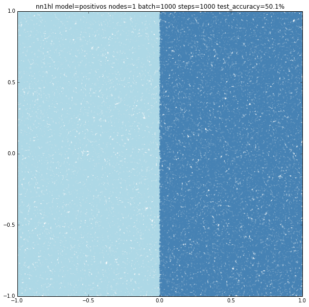
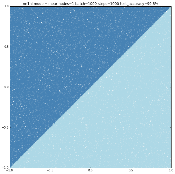
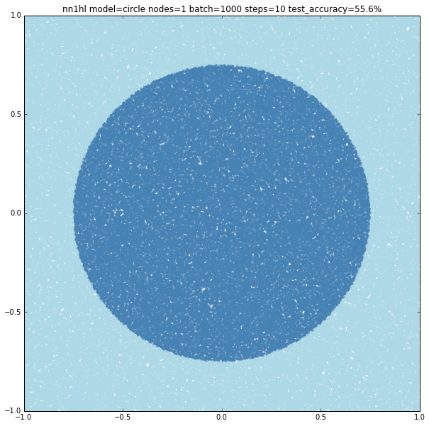

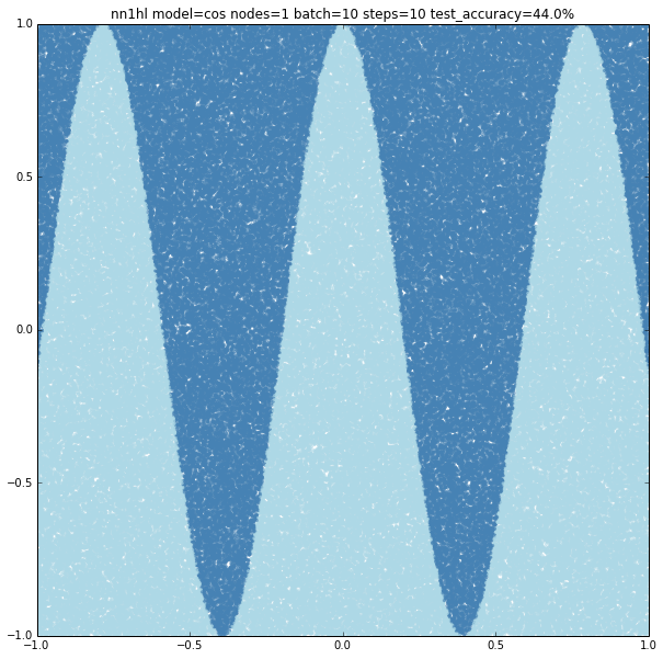
The plots shown above are generated from the training sets by setting positive samples as dark blue and negative samples as light blue.
Two neural networks are defined on the code, with a single hidden layer and with two hidden layers. Several parameters may be adjusted for each run:
Other parameters are treated as globals such as the size of the training, validation and test sets. When the NN function is called the network is trained and tested, and the predictions are added to the plot marking them on gray if the prediction was correct and on red if the prediction as incorrect in order to see where the classifier is missing it.
You can call the NN function varying the parameters to test what happens. It’s also included some iterative code to test many variants and generate a *lot* of plots. Check the code and comment what you find.
Here are some interesting results I’ve got:
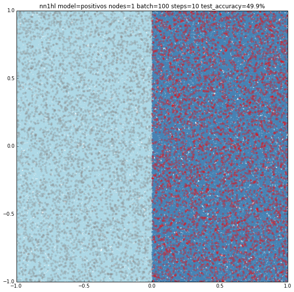
As expected, the model is too simple to really learn anything: it’s basically classifying everything as negative and thus gets a accuracy of 49.9%
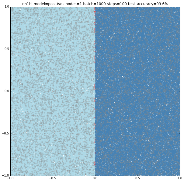
By increasing the size of the batches and steps for the stochastic gradient descent even a single node on the hidden layer yields good results: 99.6% accuracy
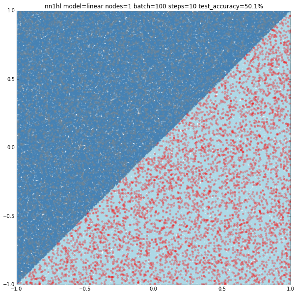
Of course few training data does anything good for a slightly more complex model: 50.1% accuracy.
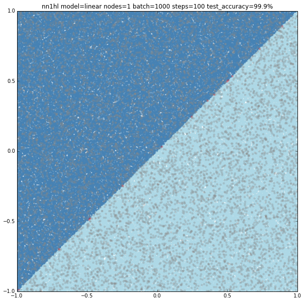
Again the classifier performs way better: 99.9%
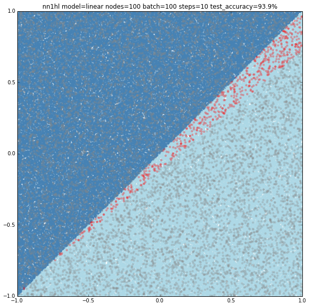
Can hidden nodes compensate for few training samples? 100 nodes, batch of 100 and 10 steps does certainly better at 93.9% accuracy and an interesting plot with linear classification on a wrong (but close) slope.
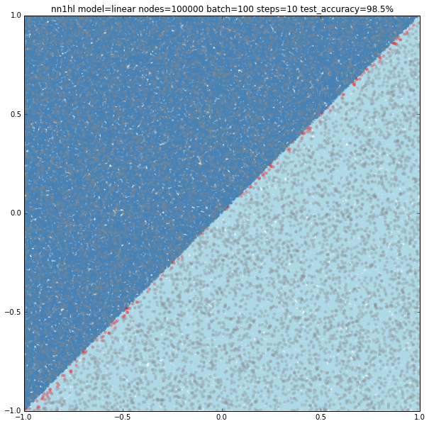
What about 1000 hidden nodes and same parameters as before? It certainly gets you closer but not still on it: 98% accuracy. Watching the slope, one can think it may be overfitting.

First tried 10,000 hidden nodes (got 98.9%) and then 100,000 nodes (shown below) and accuracy jumped back to 98.5%, clearly overfitting. For this case, a wider network behaves better but just to a certain point.
Training the classifier that previously behaved well with the circular model shows clearly it needs more data or nodes.

Turns out that it seems a single node can’t capture the complexity of the model. Varying the training parameters looks that the NN is always trying to adjust a linear classifier.
With two nodes the model looks like fitting two linear classifiers. Even varying the training parameters results are similar, except in some cases with more training data that looks like the last examples of single node (maybe overfitting?)
Using three nodes things become interesting. For a batch size of 100 and 1000 steps the NN gives a pretty good approximation to the circle and goes beyond adjusting 3 linear classifiers. Something similar happens varying the training parameters.

Increasing the number of nodes increases the precision and the visual adjustment to the circle. Check for 10 (97.8%), 100 (99%) and seems to stop at some point 1000 (99%)
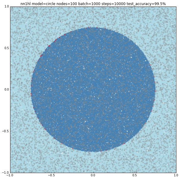
Finally increasing the training parameters on the best classifier gives us a nice 99.5% accuracy, but not sure if it’s overfitting
For the ring I started testing one of the best performers on the circle: 100 nodes, batch size of 100 and 1000 steps. Somehow expected, it tried to adjust to a single circle and missed the inner one.

Increasing the training parameters gave an interesting and unexpected result:
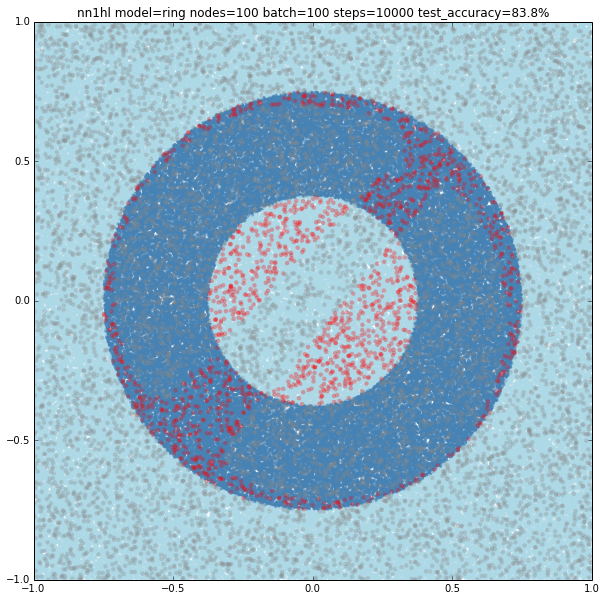
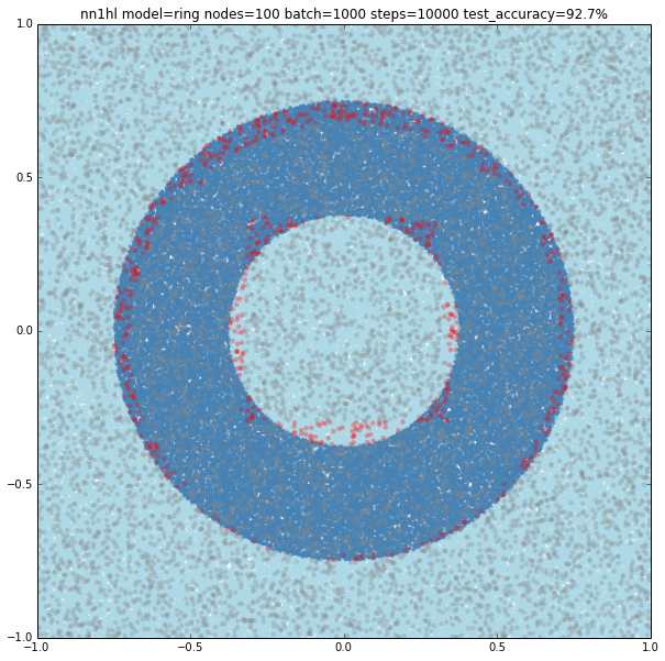
I also found that running many times with the same parameters may yield to different results. Both cases could be explained by the random initialisation and the stochastic gradient descent as the last example looks like a local minimum. Check below another interesting result using the exact same parameters yielding a pretty accurate classifier (92.7%)
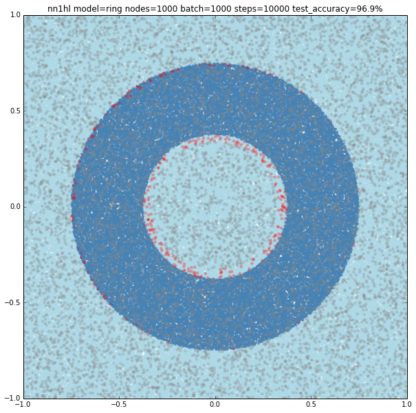
Increasing the number of nodes and the training parameters improves accuracy and makes more likely to get a classifier with a pretty good level of accuracy (96.9%). Shown below, 1000 nodes, batch size of 1000 and 10000 steps.
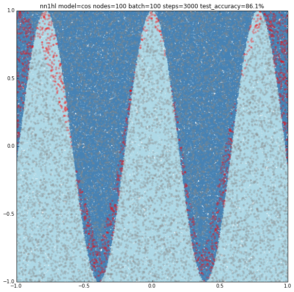
With few nodes and different training parameters we see the classifier struggling to fit.
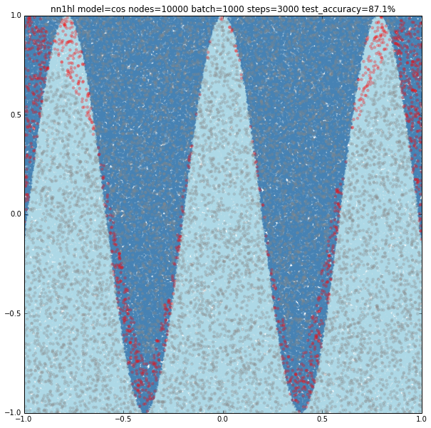
Increasing the parameters gives a model that doesn’t increase very much the accuracy (around 87%). From the ring and the cosine it looks like there are limits to the complexity a single hidden layer can handle.
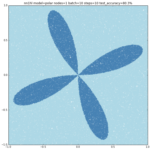
This example came as a way to try a harder problem for a classifier. As expected, the most basic versions of the parameters yield bad results. Just keep in mind that a trivial classifier that labels everything as negative would have about 80% accuracy.
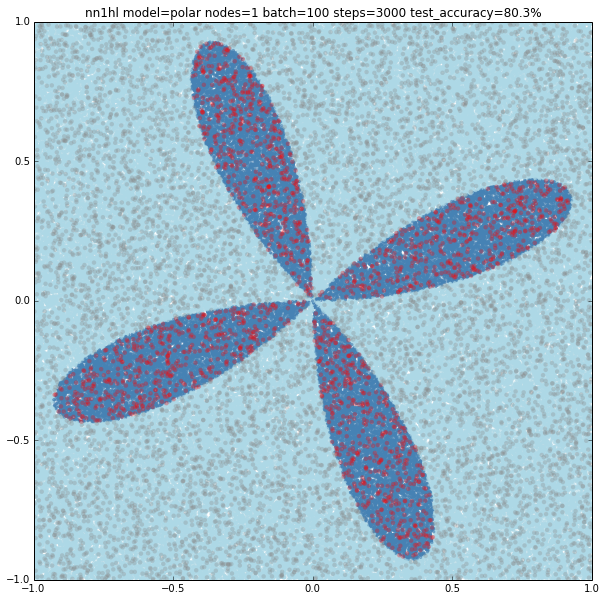
We can see that a NN with 10 nodes tries to adjust a central area as positive. Results are bad but we can see what the NN is trying to do. Increasing to 100 nodes give very similar results.
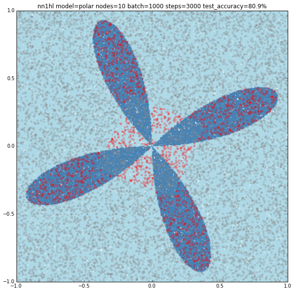
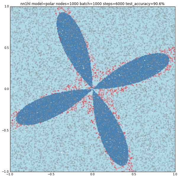
With 1000 nodes the classifier improves accuracy but misses big on the center of the model. But going up to 10,000 nodes does not improve much more. This makes me think that, as with the case of the rectangular cosine, there is a limit on what a single layer neural network may model for the classifier, and that more complex distributions may need a different kind of network.

Next I was interested in what happens with deeper networks, expanding the exercises from the Udacity course to a 3 layer NN and testing with the same models.
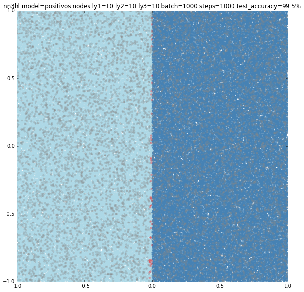
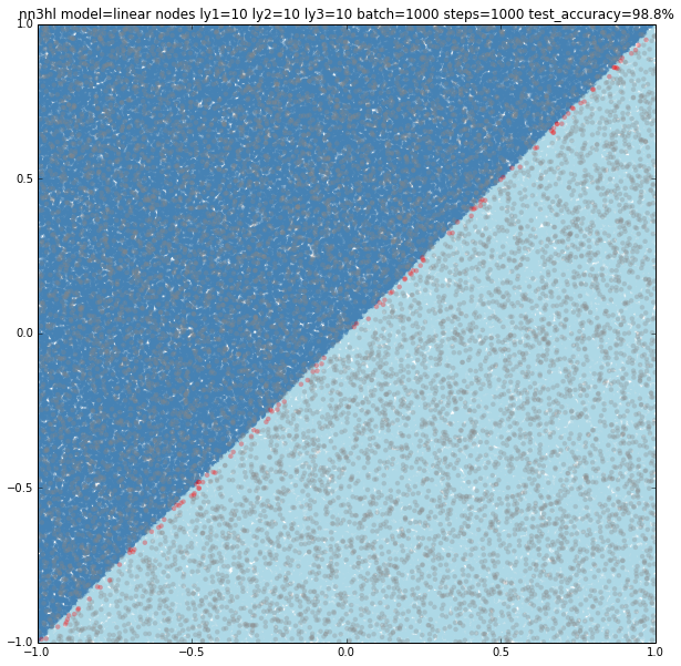
First finding was that for the Positivos example the NN needed to be of at least 10 nodes on each layer to get good results. Same classifier also worked well for the linear model, but not with the circle.
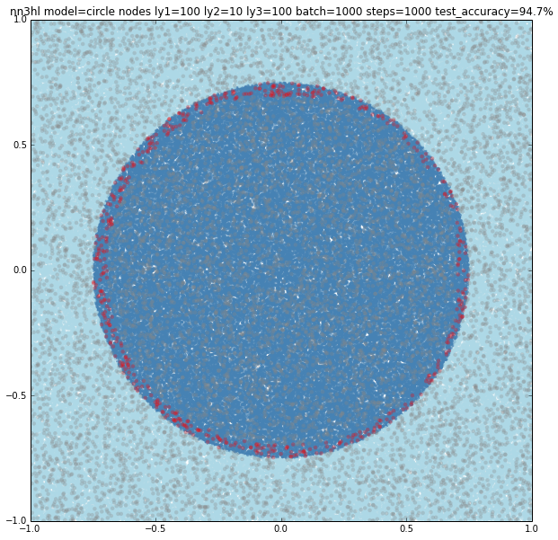
The circle needed quite an amount of nodes in some of the layers to get over 99% accuracy. The simplest model I could find with a 99.4% was (10,1000,1000) nodes. Other models with a similar count of nodes gave similar results. Models with less nodes failed completely or gave increasing accuracies.

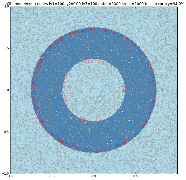
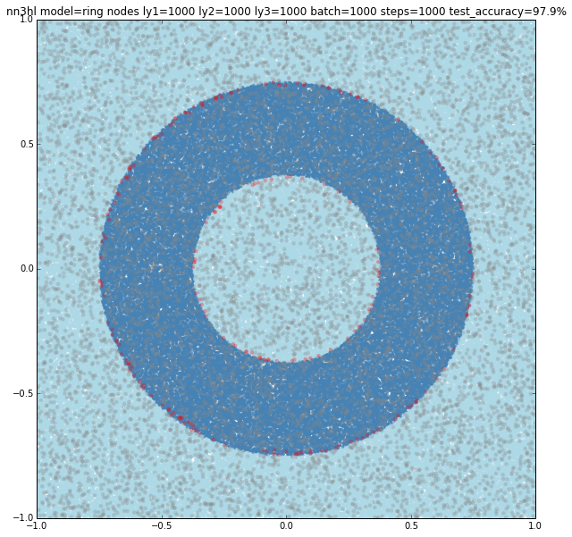
Interestingly, the ring also converged faster with (100,100,100) nodes with a 94% accuracy up to a nice 97.9% accuracy for a (1000,1000,1000) configuration.
The cosine also improved with the deeper network achieving a 94.3% accuracy with a (1000,1000,100) network. What is also interesting is that models learned by the deep network approached better than the wide network almost from the beginning. If you want to check, run the iterative version you can find commented on the code.
The most interesting case is the polar cosine on the deep network as it looks like a really hard classification problem. Base accuracy is about 80.3% for the all negative classification. As we grow the number of nodes in the different layers interesting patterns appear as you can see in the examples below.
The last example does a pretty good job classifying this complex model with a 98.1% accuracy with the three layers and 1000-1000-1000 nodes.
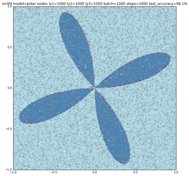
I find very interesting seeing how the wide neural network seems to have a limit on the complexity of the classifier it can learn. And the deep network looks like being able to capture that complexity. Check the Jupyter notebook at Github. You will need Tensorflow installed to run it.
Fork on Github
Kaggle’s NOAA Right Whale Recognition Challenge aims to develop an algorithm to identify individuals of Right Whales, which are critically endangered. It is a great chance to study machine learning and digital image processing although looks to me as a really hard challenge. Anyway I’ve developed this method to detect the whale in the photograph and I’m releasing it in a hope that it may help others.
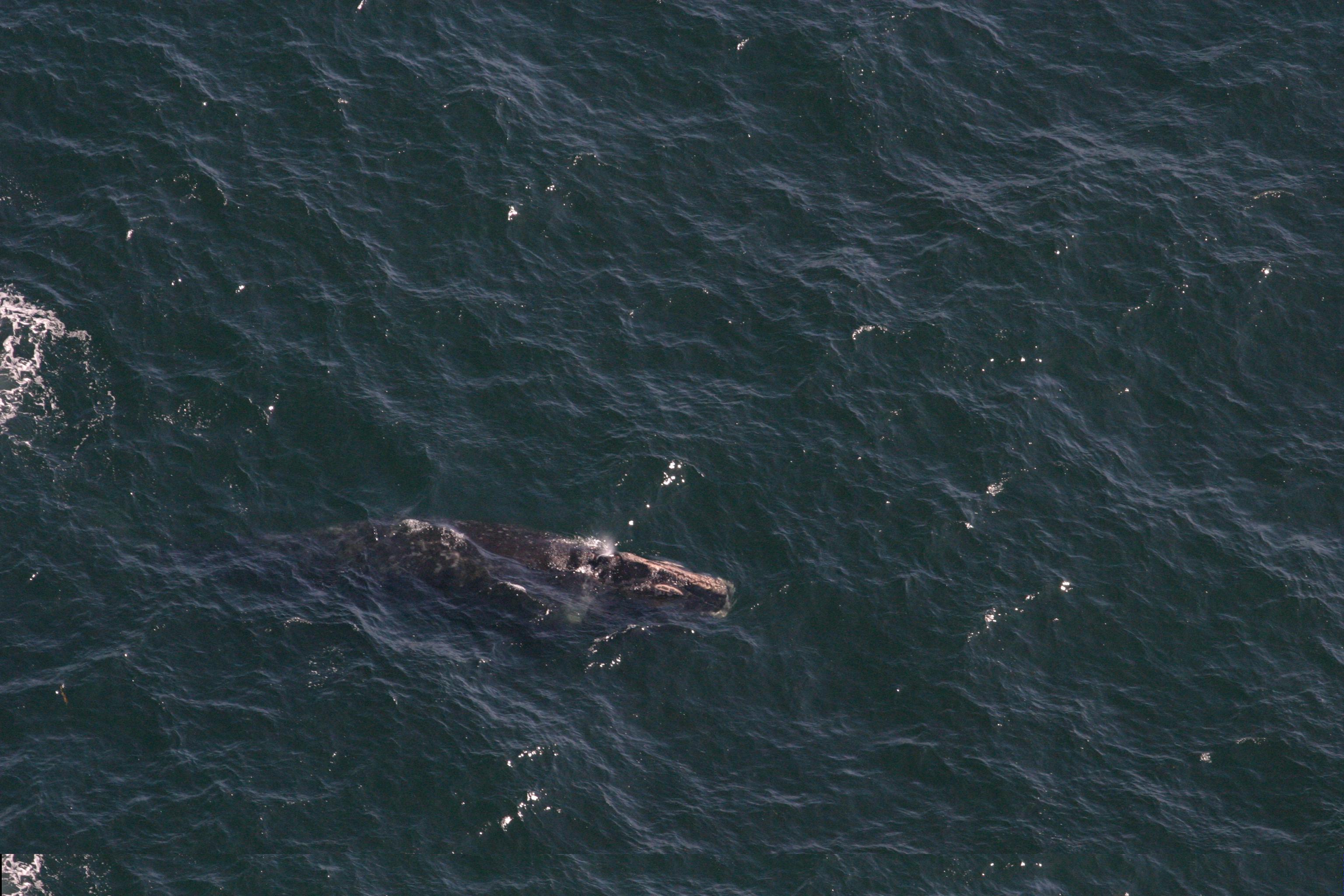
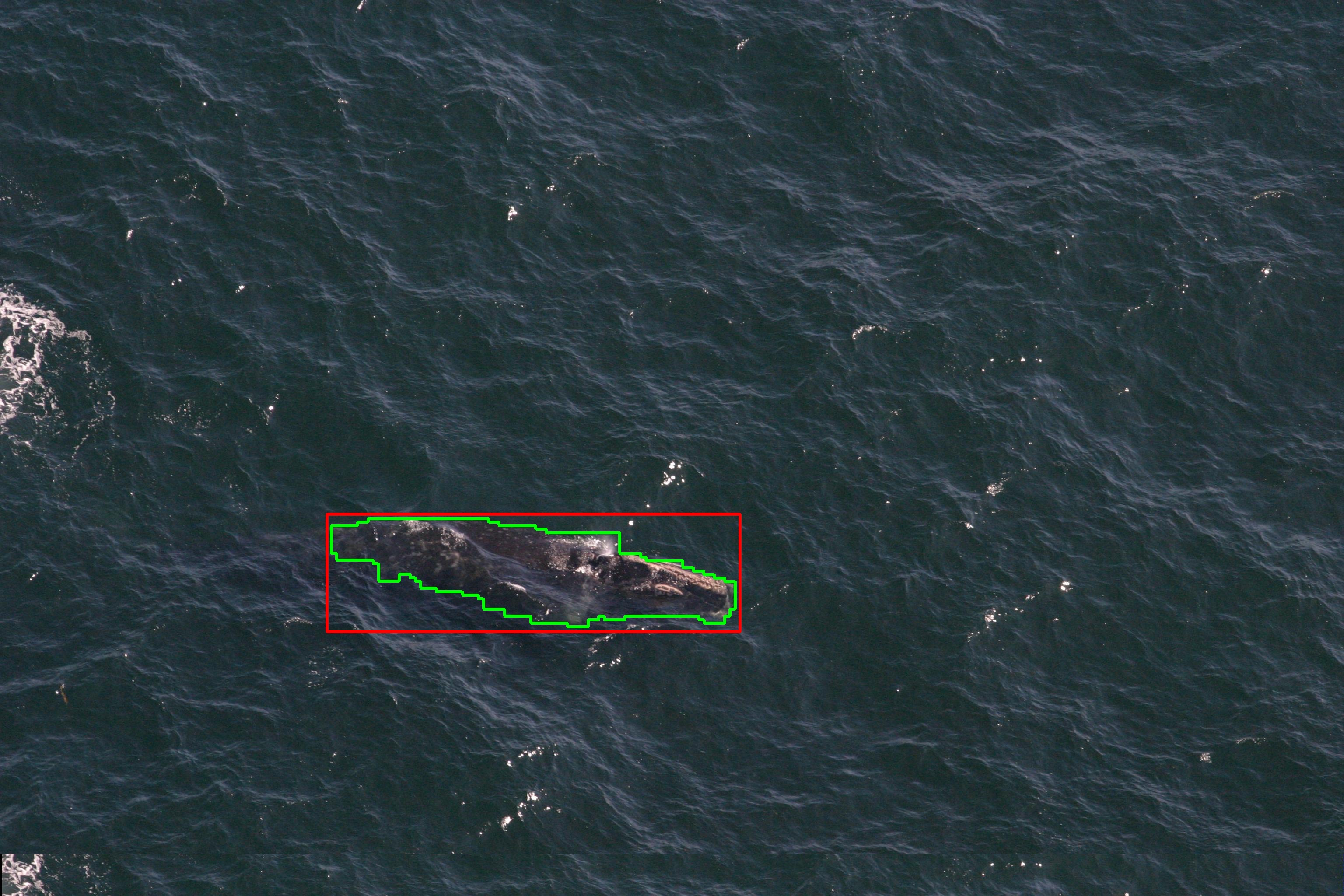
It takes advantage of the fact that most pictures are pretty plain, with almost all of the area covered by water, and have a smaller region of interest which corresponds to the whale, so the histogram for most of the image will be similar except on the region of interest. The algorithm looks recursively to subimages that have an HSV histogram not similar to the original image’s histogram, marking those regions in white and else on black. Then searches for the biggest continuous region using contours and places a bounding box around it, assuming it’s the whale. The image is called “extract” and is saved along the black & white mask.
Check the code in Github. Uses Python 2.7 and OpenCV 3.0.
Original Image:
Whale found:
Areas found mask:
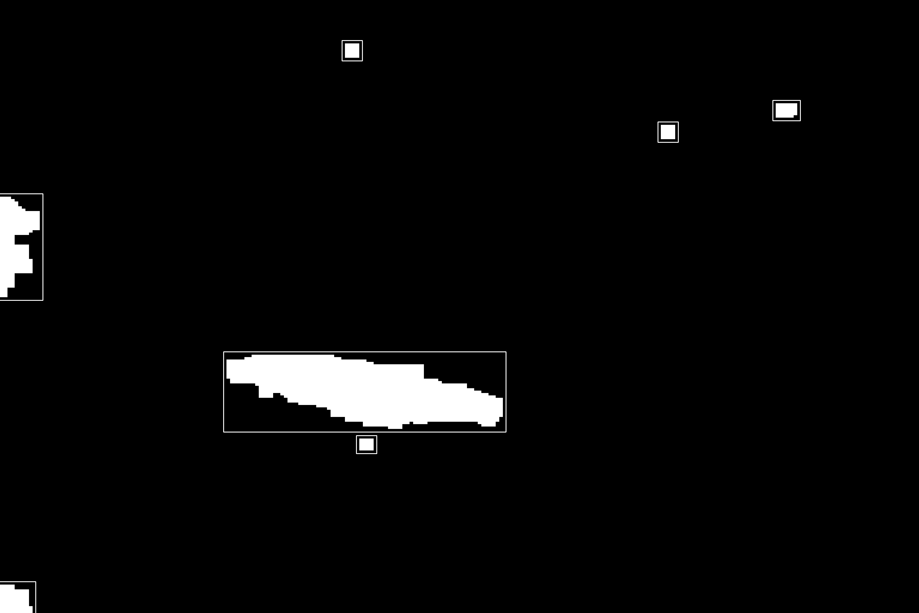
ROI Mask:

ROI Extract:

Recently I’ve been playing with Arduino, Scratch and the 3pi robot for a personal project that I hope will be interesting enough to show soon. (I’ve got a lot of motivation from these guys specially the little one with big eyes).
To start I made this little example of a RGB Led. Usually you begin making a loop through the RGB scale of colors. But it doesn’t look very natural since you expect to loop through a color hue. What you need is to convert a HSV (Hue Saturation Value) scale to RGB (Red Green Blue) scale that the LED support, and then loop through the Hue domain mantaining the Saturation and Value constants.
Circuit is here, look for the RGB LED example
Video:
Code (I’ve coded it as close as I could to the Arduino sample guidelines).
UPDATE (2019-08-21): Check repository at Github
/*
 * Color Wheel LED
 *
 * Loops a RGB LED attached to pins 9,10,11 through
 * all the "exterior" colors of a Color Wheel
 *
 * The RGB LED uses a 3 component (red green blue) model which adds light colors to produce
 * a composite color. But the RGB does not make easy to loop through a more
 * "natural" sequence of colors. The HSV (hue saturation value) model uses a color cylinder
 * in which each color is a point inside the cylinder.
 * The hue is represented by the angle at which the point is, the saturation represents
 * the length (how close to the center the point is) and the value represent the height at
 * which the point is.
 *
 * By cycling the hue value from 0 to 360 degrees, and keeping the saturation and value at 1
 * we can represent all the brightest colors of the wheel, in a nice natural sequence.
 *
 * The algorithm to convert a HSV value to a RGB value is taken from Chris Hulbert's blog (splinter)
 *
 * Created 1 January 2011
 * By Eduardo A. Flores Verduzco
 * http://eduardofv.com
 *
 * References:
 * http://en.wikipedia.org/wiki/HSL_and_HSV
 * http://en.wikipedia.org/wiki/Color_wheel
 * http://splinter.com.au/blog/?p=29
 *
 *
 */

void setup() {
  //Set the pins to analog output
  pinMode(9,OUTPUT);
  pinMode(10,OUTPUT);
  pinMode(11,OUTPUT);
}

void loop() {
  //The Hue value will vary from 0 to 360, which represents degrees in the color wheel
  for(int hue=0;hue<360;hue++)
  {
    setLedColorHSV(hue,1,1); //We are using Saturation and Value constant at 1
    delay(10); //each color will be shown for 10 milliseconds
  }
}

//Convert a given HSV (Hue Saturation Value) to RGB(Red Green Blue) and set the led to the color
//  h is hue value, integer between 0 and 360
//  s is saturation value, double between 0 and 1
//  v is value, double between 0 and 1
//http://splinter.com.au/blog/?p=29
void setLedColorHSV(int h, double s, double v) {
  //this is the algorithm to convert from RGB to HSV
  double r=0;
  double g=0;
  double b=0;

  double hf=h/60.0;

  int i=(int)floor(h/60.0);
  double f = h/60.0 - i;
  double pv = v * (1 - s);
  double qv = v * (1 - s*f);
  double tv = v * (1 - s * (1 - f));

  switch (i)
  {
  case 0: //rojo dominante
    r = v;
    g = tv;
    b = pv;
    break;
  case 1: //verde
    r = qv;
    g = v;
    b = pv;
    break;
  case 2:
    r = pv;
    g = v;
    b = tv;
    break;
  case 3: //azul
    r = pv;
    g = qv;
    b = v;
    break;
  case 4:
    r = tv;
    g = pv;
    b = v;
    break;
  case 5: //rojo
    r = v;
    g = pv;
    b = qv;
    break;
  }

  //set each component to a integer value between 0 and 255
  int red=constrain((int)255*r,0,255);
  int green=constrain((int)255*g,0,255);
  int blue=constrain((int)255*b,0,255);

  setLedColor(red,green,blue);
}

//Sets the current color for the RGB LED
void setLedColor(int red, int green, int blue) {
  //Note that we are reducing 1/4 the intensity for the green and blue components because
  //  the red one is too dim on my LED. You may want to adjust that.
  analogWrite(9,red); //Red pin attached to 9
  analogWrite(10,green/3); //Red pin attached to 9
  analogWrite(11,blue/3); //Red pin attached to 9
}