When transforming vectors to their Principal Components, are their relations preserved?


pca test


Question: When transforming vectors to their Principal Components, are their relations preserved?

We have a set of vectors. After performing Principal Component Analysis (PCA) we now use the “rotated” vectors to perform analysis. Can we be confident that the original relations (cosine similarity between vectors) are preserved on the new vector space?

knitr::opts_chunk$set(echo = TRUE)
set.seed(1234)
#Cosine Similarity
cos.sim <- function(A,B) 
{
  return( sum(A*B)/sqrt(sum(A^2)*sum(B^2)) )
}   

1 – Generate a test set y=x+err

#"noisy" x=y
x = runif(n = 1000,min=-100,max=100) # x has a uniform distribution
y = x + rnorm(n=1000,mean=0,sd=20) # y has a normal distribution

d <- data.frame(x=x,y=y)
#ver primeros puntos
head(d)
##           x            y
## 1 -77.25932 -57.56371837
## 2  24.45988  -0.03487656
## 3  21.85495  36.04947094
## 4  24.67589  22.49148848
## 5  72.18308 107.83523462
## 6  28.06212  23.19322747
plot(d)

2 – Perform PCA

pca <- prcomp(d,center = F,scale. = F)
summary(pca)
## Importance of components:
##                           PC1      PC2
## Standard deviation     83.040 13.30478
## Proportion of Variance  0.975  0.02503
## Cumulative Proportion   0.975  1.00000
pca$rotation
##        PC1       PC2
## x 0.691987 -0.721910
## y 0.721910  0.691987
dt <- pca$x #d transformed
head(dt)
##            PC1        PC2
## [1,] -95.01826  15.940928
## [2,]  16.90074 -17.681966
## [3,]  41.14781   9.168461
## [4,]  33.31222  -2.249953
## [5,] 127.79708  22.510896
## [6,]  36.16204  -4.208914
plot(dt)

3 – For a given vector, calculate it’s relation (cosine similarity) to all the others in both spaces

a <- d[2,] #choose a point on the original space
s<-apply(d,1,function(x) cos.sim(a,x)) #calculate the angles to all the other vectors
at <- dt[2,] #get the same point in the new space
st<-apply(dt,1,function(x) cos.sim(at,x)) #calculate the angles in the new space

The angles are the same

head(data.frame(s=s,st=st))
##            s         st
## 1 -0.8010403 -0.8010403
## 2  1.0000000  1.0000000
## 3  0.5171996  0.5171996
## 4  0.7381007  0.7381007
## 5  0.5550765  0.5550765
## 6  0.7698978  0.7698978

Check closest points are the same

head(data.frame(s=order(s,decreasing = T),st=order(st,decreasing = T)))
##     s  st
## 1   2   2
## 2 898 898
## 3 387 387
## 4  47  47
## 5 571 571
## 6 299 299

Answer: YES

4 – Bonus: magnitudes are also the same

magd <- sqrt(rowSums(d*d))
magdt <- sqrt(rowSums(dt*dt))

head(data.frame(magd=magd,magdt=magdt))
##        magd     magdt
## 1  96.34617  96.34617
## 2  24.45991  24.45991
## 3  42.15689  42.15689
## 4  33.38812  33.38812
## 5 129.76453 129.76453
## 6  36.40616  36.40616

5 – Bonus: you can retreive the distributions

hist(as.data.frame(dt)$PC1) #this is close to uniform

hist(as.data.frame(dt)$PC2) #this is close to normal

Looks closer than the original x,y

hist(d$x)

hist(d$y)


Stacked and Grouped Barplots in R

Fork on github
This is a modified version of the original barplot in the R core that lets you add more series as stacked and grouped by adding trailing space with space and a new space-before parameters.

barplot.sg(m3,space.before=0,space=2.5, col=pal1, ylim=c(0,1.2*max(m1[2,])), border=NA)
barplot.sg(m2,space.before=1,space=1.5, col=pal2 ,xaxt="n", border=NA, add=T)
barplot.sg(m1,space.before=2,space=0.5, col=pal3,xaxt="n", border=NA, add=T)
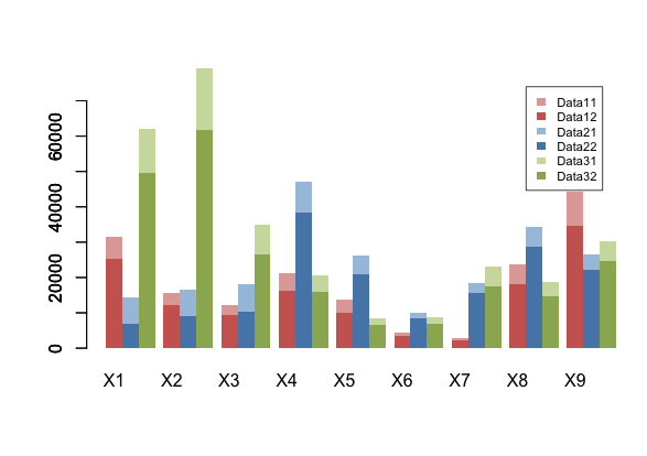
stacked and grouped barplot