MeLi Data Challenge 2019 – Multiclass Classification in Keras

The MercadoLibre Data Challenge 2019 was a great competition Kaggle’s style with an awsome prize consisting on tickets (and accomodation & air tickets) to Khipu Latin American conference on Artificial Intelligence.

I gave it a try implementing several ideas I already had in my head. First I tried a standard BERT embeddings classifier which proved harder to implement in Keras with all the current changes that have been going on with Tensorflow 2.0. Next I tried a Multi Layer Perceptron (MLP) fed with fixed BERT precalculated sentence embeddings. These two approaches didn’t traveled too far but may be interesting starting points to try in the future.

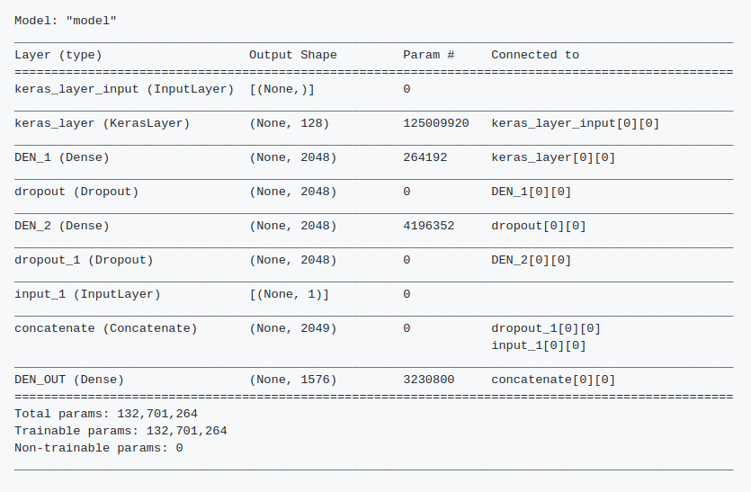
Finally a simpler model gave me the best results I could get, with a Balanced Accuracy Score of 0.87, which put me in the 45st place in the leaderboard. The model uses a Tensorflow Hub Keras layer fine tunned from Neural Probabilistic Language Model described here, followed by a MLP, trained with Adam and Sparse Categorical Crossentropy loss. Check the Github repository for details and code.

Some interesting findings:

  • The language model that I used was spanish based but performed almost equally well in portuguese (nnlm-es-128dim-with-normalization)
  • I got slightly better results by training the same model separetly on both languages and merging the results. But a single model trained on the whole dataset perfomed almost as well

The kind guys at MercadoLibre did a kickstart workshop and gave away a model that uses ULMFiT and reaches also 0.87. I think it’s very interesting that my model, using a different approach reaches a very similar result, and that’s why I’m pretty happy with it despite being very far from the first places!

When transforming vectors to their Principal Components, are their relations preserved?


pca test


Question: When transforming vectors to their Principal Components, are their relations preserved?

We have a set of vectors. After performing Principal Component Analysis (PCA) we now use the ā€œrotatedā€ vectors to perform analysis. Can we be confident that the original relations (cosine similarity between vectors) are preserved on the new vector space?

knitr::opts_chunk$set(echo = TRUE)
set.seed(1234)
#Cosine Similarity
cos.sim <- function(A,B) 
{
  return( sum(A*B)/sqrt(sum(A^2)*sum(B^2)) )
}   

1 – Generate a test set y=x+err

#"noisy" x=y
x = runif(n = 1000,min=-100,max=100) # x has a uniform distribution
y = x + rnorm(n=1000,mean=0,sd=20) # y has a normal distribution

d <- data.frame(x=x,y=y)
#ver primeros puntos
head(d)
##           x            y
## 1 -77.25932 -57.56371837
## 2  24.45988  -0.03487656
## 3  21.85495  36.04947094
## 4  24.67589  22.49148848
## 5  72.18308 107.83523462
## 6  28.06212  23.19322747
plot(d)

2 – Perform PCA

pca <- prcomp(d,center = F,scale. = F)
summary(pca)
## Importance of components:
##                           PC1      PC2
## Standard deviation     83.040 13.30478
## Proportion of Variance  0.975  0.02503
## Cumulative Proportion   0.975  1.00000
pca$rotation
##        PC1       PC2
## x 0.691987 -0.721910
## y 0.721910  0.691987
dt <- pca$x #d transformed
head(dt)
##            PC1        PC2
## [1,] -95.01826  15.940928
## [2,]  16.90074 -17.681966
## [3,]  41.14781   9.168461
## [4,]  33.31222  -2.249953
## [5,] 127.79708  22.510896
## [6,]  36.16204  -4.208914
plot(dt)

3 – For a given vector, calculate itā€™s relation (cosine similarity) to all the others in both spaces

a <- d[2,] #choose a point on the original space
s<-apply(d,1,function(x) cos.sim(a,x)) #calculate the angles to all the other vectors
at <- dt[2,] #get the same point in the new space
st<-apply(dt,1,function(x) cos.sim(at,x)) #calculate the angles in the new space

The angles are the same

head(data.frame(s=s,st=st))
##            s         st
## 1 -0.8010403 -0.8010403
## 2  1.0000000  1.0000000
## 3  0.5171996  0.5171996
## 4  0.7381007  0.7381007
## 5  0.5550765  0.5550765
## 6  0.7698978  0.7698978

Check closest points are the same

head(data.frame(s=order(s,decreasing = T),st=order(st,decreasing = T)))
##     s  st
## 1   2   2
## 2 898 898
## 3 387 387
## 4  47  47
## 5 571 571
## 6 299 299

Answer: YES

4 – Bonus: magnitudes are also the same

magd <- sqrt(rowSums(d*d))
magdt <- sqrt(rowSums(dt*dt))

head(data.frame(magd=magd,magdt=magdt))
##        magd     magdt
## 1  96.34617  96.34617
## 2  24.45991  24.45991
## 3  42.15689  42.15689
## 4  33.38812  33.38812
## 5 129.76453 129.76453
## 6  36.40616  36.40616

5 – Bonus: you can retreive the distributions

hist(as.data.frame(dt)$PC1) #this is close to uniform

hist(as.data.frame(dt)$PC2) #this is close to normal

Looks closer than the original x,y

hist(d$x)

hist(d$y)