Stacked and Grouped Barplots in R

Fork on github
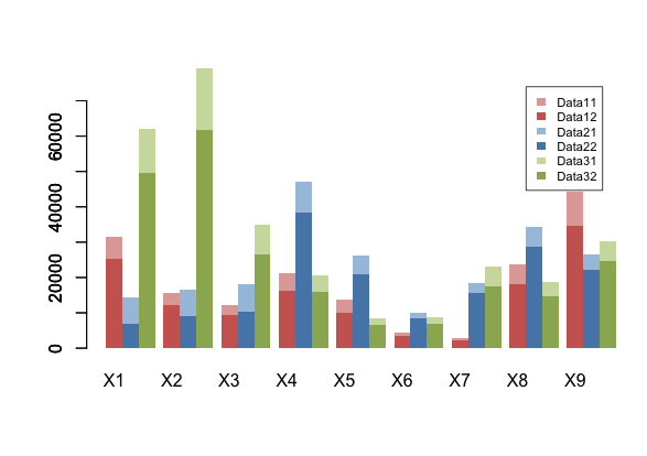
This is a modified version of the original barplot in the R core that lets you add more series as stacked and grouped by adding trailing space with space and a new space-before parameters.

barplot.sg(m3,space.before=0,space=2.5, col=pal1, ylim=c(0,1.2*max(m1[2,])), border=NA)
barplot.sg(m2,space.before=1,space=1.5, col=pal2 ,xaxt="n", border=NA, add=T)
barplot.sg(m1,space.before=2,space=0.5, col=pal3,xaxt="n", border=NA, add=T)

stacked and grouped barplot

Arduino sample: Heartbeat

I’ve written a small sketch for Arduino to make a led blink with a function that resembles a human heartbeat. 

On [1] Stevens and Lakin describe a detailed mathematical analysis of the signal of the cardiac pulse. 

I’ve taken one of their equations that close to the cardiac pulse and generated a lookup table for the luminosity value.

  f(x)=(sin(x)^13) * cos(x-PI/10)

  check the function graphed on Google 

Check the code at Github.

[1] Stevens, Scott; Lakin, William. A Differentiable, Periodic Function for Pulsatile Cardiac 

    Output Based on Heart Rate and Stroke Volume

    http://math.bd.psu.edu/faculty/stevens/Publications/paper3.pdf


DIY Raspberry Pi Cobbler (for the GPIO)

The Adafruit Raspberry Pi Cobbler is a nice breakout for the Raspberry Pi GPIO designed to connect to a breadboard. While not expensive (US$7.95) shipping simple electronic devices to Mexico can double it’s price due shipping and it may take several weeks to be delivered. So I decided to make one from components I could get easily here.

Components:

  • 25 cms of 26 pin ribbon cable
  • Two female 26 headers for ribbon cable (press connectors)
  • One generic protoboard
  • One strip of break away headers with 26 pins
  • One strip of break away headers with 26 double pins

First, build the ribbon cable following Gert’s instructions.

Now, take a look at the protoboard I got from Steren. Looks like a solderless breadboard. Notice that each row the left side of the vertical tracks has two single point pads while the right side has three. I used the side with two pads, and inserted the row of double pins on them. The ribbon cable will be connected to this headers.

The protoboard. Notice the 2 single pads side and the 3 single pads side on each row

The double pin header row. It’s position corresponds to the two single pads

The single pin headers will connect the protoboard with the breadboard. As this terminals have to be longer and must be soldered on the copper side of the breadboard, I inserted them upside down and then pushed them from the top just to the plastic to make them as long as they can on the bottom side.

The single pin headers inserted upside down. Check the three leftmost pins that have been pushed down further.

Given the odd layout of the protoboard, I found easier to put the right side headers one hole farther and put jumpers between the tracks. Check how the solder bridges the up and down facing pins and tracks.


The jumpers on the up side and the soldering on the down side.

Finally, cut it using a Dremel. I should have done this before the soldering!.

Side view.

A Laser Range Finder using RapsberryPi, Arduino and OpenCV

I’ve been working on a project to build a Laser Range Finder using a Raspberry Pi, an Arduino and OpenCV using a webcam. I hope that eventually this project may be used on a mobile robot using the algorithms taught on Udacity CS373 specially SLAM (Synchronous Location and Mapping).

The First Prototype

This first protoype is more a proof of concept than a usable device. Anyway, it’s working pretty well except for it being quite slow.

  • Raspberry Pi Model B running:
    • Archlinux ARM with a modified kernel to support the Arduino and the Webcam
    • OpenCV 2.4.1
    • Python 2.7
    • The LRF software
  • Arduino UNO connected via USB to the Raspberry Pi. Runs a controller that receives a message to turn on and off the laser. I hope it will also control some servos later.
  • A Logitech c270 webcam, disassembled, so it can be installed on the casing
  • Sparkfun TTL Controlled Laser Module
  • A targus mini USB hub
  • My Powered USB cable to provide the extra current that the Raspberry Pi can’t provide to the USB devices
  • A couple of USB power sources, one for the RPi and the other for the USB devices
  • A lousy acrylic casing, the first thing I’ve done with acrylic

Also check the video for an overview on it’s parts and how it works.

This prototype is very slow (one measurement takes about 10 seconds) but I’m optimistic that it may become more functional on a couple of iterations, specially with the upcoming Raspberry Pi Foundation CSI camera. The device is pretty accurate and precise on short distances but, as expected, both decrease at large distances. I would estimate that from a distance up to 35cms it’s very accurate, from 35 to about 60cms has pretty good and up to 2m it may be good enough for a small robot.Later I’ll post more details on the measured precision and accuracy and some tricks to enhance them.

As you can see on the video, it has a simple web interface to trigger the measurement process. It can also be done command line by SSHing to the Raspberry Pi. I’ll also post how OpenCV detects the laser in the image, and the next steps I’ll take to improve. For now you can get most of the working code from Github. The details of the mathematical model appears below.

All comments are welcome here (comments section at the bottom) or via Twitter.

The Model

This diagram shows the basic idea for the project. The laser is shot to a target at a known angle and the image is captured on the webcam. The angle at which the laser appears on the image corresponds to the incidence angle of the laser at the target, and thus, to the distance to the target.

If the target is a little farther, so that the laser crosses the focus line of the camera, the model is a bit different:

Here we are considering that both the camera-to-laser angle (β) and the distance from the camera to the laser (L) are fixed. We also know the focal distance (f) and the horizontal resolution (CAMERA_WIDTH) that are parameters of the camera. With OpenCV we can process the image and calculate the horizontal distance (vc) from the camera’s Y axis to the point where the laser appears on the image. Given those values we can use simple trigonometry to calculate the angle at which the laser appears on the image (δ) and the distance from the camera to the target (Dc). Note that we are looking Dc and not D which is the perpendicular distance from the camera to the target. By the way, for the purposes of this model the webcam is considered a pinhole camera. Later on we will correct the physical camera to adjust the model.

vx = CAMERA_WIDTH – vc
δ = atan( f / vx )
λ = π – β – δ
Dc = L * sin( β / λ )

I’ll post later details on the implementation.

Visualización: Movilidad Laboral en México

Seguimos analizando el comportamiento del los candidatos que buscan empleo en OCCMundial. En esta ocasión recreamos una visualización que hicimos hace mas de un año sobre las “rutas” que se generan cuando la gente solicita empleo fuera de la zona donde reside. Para ello obtuvimos un conjunto de datos de 48,801 solicitudes de empleo anonimizadas, marcadas con las direcciones de origen (la del candidato) y destino (de la vacante según lo capturado por el reclutador). Para obtener las coordenadas geográficas de ambos puntos usamos el API de Google Maps al cual le enviamos las direcciones lo más limpias posible y obtuvimos la coordenadas más próximas que Google pudo encontrar. Estos datos los graficamos en un mapa en forma de curvas de llegada/salida en Processing usando el método para mapas georeferenciados que describí hace algún tiempo usando mapa blanco con líneas negras de este otro post.

En la visualización se pueden ver las principales ciudades de México ligadas mediante curvas. Cada curva tiene un origen, es decir, un punto de dónde un candidato está solicitando un empleo, y un destino, el lugar donde se está ofreciendo la vacante. En el punto de origen la linea tiene una mayor curvatura y en el destino llega casi recta. Por ejemplo, en la siguiente imagen se muestra la zona de Puerto Vallarta (derecha) y Guadalajara (derecha) donde se puede ver dos cosas: que a Guadalajara llega y se va mucho mas gente que en Puerto Vallarta, pero que al mismo tiempo mucho mas gente quiere ir de Guadalajara a Puerto Vallarta que a la inversa.

Desarrollamos también una visualización inteactiva que permite observar mejor las rutas de llegada y salida. Al colocar el mouse en alguna ciudad se resaltan las rutas de salida en azul y las de llegada en verde. El nombre y las cantidades se muestran en la esquina inferior izquierda. La visualización está hecha en Processing.js y requiere un browser con soporte de HTML 5. El proceso es un poco lento ya que cada vez que se selecciona una ciudad se recalculan las 48000 rutas para mostrar solo las relevantes. Funciona en iPad pero requiere un poco de paciencia.

Hay algunas consideraciones necesarias de tomar en cuenta al usar esta herramienta:

  • En muchas ocasiones no se cuenta con direcciones exactas, por lo que se aproximan lo más posible.
  • Cuando solo se tiene información a nivel estado, se las rutas se dirigen a un punto central en ese estado. Por ejemplo, en Baja California ese punto se encuentra entre Mexicali y Tijuana, un poco al sur.
  • Hay errores en algunos nombres de localidades, si encuentras alguno, por favor házmelo saber.
  • Los nombres de ciudades no tienen acentos.


El Diseño Gráfico es obra de @marco_aom, ¡muchas gracias!

¡Todos los comentarios son bienvenidos, por Twitter o en este blog!

Images licensed under Creative Commons Attribution 3.0 Unported. These files are licensed under the Creative Commons Attribution 3.0 Unported license: You are free: to share, to copy, distribute and transmit the work to remix or to adapt the work Under the following conditions: attribution: You must attribute the work in the manner specified by the author or licensor (but not in any way that suggests that they endorse you or your use of the work). Code is OpenSource under MIT License.

OpenCV on the Raspberry Pi with Arch Linux ARM

These are my notes on how I got OpenCV running on the Raspberry Pi today with a webcam. On this post you can find the Debian version that I did earlier.

  • Install Arch Linux ARM from image, use this guide.
  • Expand linux parition, also detailed on the same guide.
  • Configure copying arm224_start.elf to start.elf to get more memory for the apps
  • Configure networking: edit /etc/rc.conf and /etc/resolv.conf. Check this topic
  • Modify pacman configuration /etc/pacman.conf to use curl to download packages for my slow connection by uncommenting the line:
     XferCommand = /usr/bin/curl -C - -f %u > %o
  • I tried several times to update pacman and system using
    pacman -Syu

    but some errors about udev and libusb were found, and I finally gave up with this step. At last, everything worked except lxde which I don’t need, so I’ll check this back some other time.

  • Install lxde. I’m not sure if some libraries installed by this are useful to OpenCV.
    pacman -S lxde xorg-xinit xf86-video-fbdev
    
  • lxde didn’t worked: every time I tried to xinit, it throwed a error about libudev.so.1 not being found.
  • Install python2 (which was already installed but was updated), numpy, opencv and samples:
    pacman -S python2 python2-numpy opencv opencv-samples
    
  • Finally I run a simple test I use to open the webcam stream, take a frame and save it. It didn’t worked immediatly since I found that a Dell multimedia keyboard I had attached to a USB hub with my DIY USB powered cable with the webcam had some issues. But after solving it, the camera works and saves the image. The sample is this:
    import cv2.cv as cv
    import time
    
    #cv.NamedWindow("camera", 1)
    
    #capture = cv.CaptureFromCAM(-1)
    capture = cv.CreateCameraCapture(1)
    #cv.SetCaptureProperty(capture,cv.CV_CAP_PROP_FPS, 3)
    cv.SetCaptureProperty(capture,cv.CV_CAP_PROP_FRAME_WIDTH, 1280)
    cv.SetCaptureProperty(capture,cv.CV_CAP_PROP_FRAME_HEIGHT, 720)
    
    img = cv.QueryFrame(capture)
    
    print "Captured "
    cv.SaveImage("output.jpg",img)

Law of Large Numbers, Visualized

As a follow up on the post “How Common Is Your Birthday – 360 degrees” we are getting our own data from OCCMundial to compare México with the US data from the NYTimes. We made several runs with different dataset sizes and, as a byproduct of this, we got a visualization that shows how the probability distribution of the birthday rank becomes apparent as the dataset size increases.

Check the visualization and source code (in Processing.js) here.

Rank for more common birthdays along the year. Whiter is highest rank, so most common birthday. Data for a random sample of 5,000, 100,000, 1.5 million and 4.5 million records. As dataset size increases, the real distribution becomes apparent. Data from México (OCCMundial).

Visualization: How Common Is Your Birthday – 360 degrees

I’ve done a visualization based on this one by Matt Stiles. Use the mouse to locate a birth date. I’ve a added a red arc that indicates the most probable conception date for the given birth date based on an average pregnancy of 39.5 weeks. January 1st is at 0 degrees and the year goes clockwise. I think that a circle gives a better impression on what’s happening around the year. Check the gaps at some special dates likes July 4th, Christmas and Thanks Giving weeks.

I hope to have another visualization with our own data soon.

Images licensed under Creative Commons Attribution 3.0 Unported. These files are licensed under the Creative Commons Attribution 3.0 Unported license. You are free: to share, to copy, distribute and transmit the work to remix or to adapt the work Under the following conditions: attribution: You must attribute the work in the manner specified by the author or licensor (but not in any way that suggests that they endorse you or your use of the work). Code is OpenSource bajo MIT License.

DIY Powered USB Cable for Raspberry Pi

I’ve got a Logitech c270 webcam working on the Raspberry Pi with Archlinux, since the current Debian image does not include the video modules. The main issue is power. I’ve measured the current that the camera is using and it goes up to 240mA when capturing video which is well over the Pi’s specification. If you can get a powered USB hub I guess that will work, just keep an eye on the power consuption of all the devices connected to it.

I have built a powered usb cable from a USB extension cable and a USB Type A-B cable. The extension cable is the one that has on each side a Type A male and female (receptacle), and is used to access a remote USB port. The type A to B cable is the one that is commonly used to connect a host to a device, like a computer to a printer, and that seems to be used less nowadays.


USB connectors. Three right-most are: Type A female (receptacle), Type A male and Type B

Please note that doing this may be dangerous or risky for your devices, since a shortcut or an incorrectly plugged terminal may damage or blow any of them. Build this at you own risk!. Also take into account that this cable will be less reliable than the original cables.

The USB standard pinout consists of four conductors: Ground (GND – black), VBUS (+5V – red), Data+ (D+ – green) and Data- (D- – white). We will connect the GND and VBUS lines from the extension cable to the GND and VBUS lines of the Type A side of the other cable, leaving both Data lines untouched in the extension cable. The Data lines of the Type-A from the AB cable will not be used (will be unconnected). The Type-B side of the AB cable will be thrown away.

Cut the extension cable from the middle. If possible, do not touch the green and white lines. If you need to cut them, resolder both later to keep the same configuration as the original.

Cut the A-B cable and throw away the B side. Peel the red and black lines of the A side and trim the white and green lines since they will not be used. Connect and solder the red conductors of the two Type A male sides and the Type A female. Connect and solder the black conductors of the three connectors. Isolate the connections (I used thermofit). Use some electrical tape to strengthen the cable. Test using a multimeter.

You will have a cable with two Type A male connectors and one Type A female connector (receptacle).

You can now connect the cable to the devices. I recommend this order:

  • The Type-A (male) from the A-B cable to a USB power source (like a phone’s charger)
  • The Type-A (male) from the extension cable to the Raspberry Pi
  • The Type-A (female, receptable) to the device, in my case, the webcam.

Everything should run smoothly since the power for the device is now taken from the charger and not from the board.

Once again, do this at your own risk and evaluate your skills. The procedure is simple but it may produce irreversible damage to your devices if done improperly.
Installing OpenCV on the Raspberry Pi

UPDATE 2:Here is my guide for Arch Linux

UPDATE: I’ve moved to Archlinux because it has the webcam modules included. OpenCV is really easy to install: pacman -S opencv

Installing OpenCV (2.3.1) on the Raspberry Pi is pretty easy using the base Debian Squeeze image and following these instructions for Debian/Ubuntu.You will need to have more space on the root partition so I recommend resizing it to at least 3GB (see the video tutorial using GParted or follow these instructions). Here they are with some comments on the few issues I found:

I found an error trying to install cmake for the first time, so first do

sudo apt-get update

two times before anything else. The first time I did the update an error on “duplicate sources” was shown thus the second update was necessary.

Install in the following order:

sudo apt-get install build-essential
sudo apt-get install cmake 
sudo apt-get install pkg-config 
sudo apt-get install libpng12-0 libpng12-dev libpng++-dev libpng3 
sudo apt-get install libpnglite-dev libpngwriter0-dev libpngwriter0c2 
sudo apt-get install zlib1g-dbg zlib1g zlib1g-dev 
sudo apt-get install pngtools libtiff4-dev libtiff4 libtiffxx0c2 libtiff-tools 
sudo apt-get install libjpeg8 libjpeg8-dev libjpeg8-dbg libjpeg-progs 
sudo apt-get install ffmpeg libavcodec-dev libavcodec52 libavformat52 libavformat-dev 
sudo apt-get install libgstreamer0.10-0-dbg libgstreamer0.10-0  libgstreamer0.10-dev 
sudo apt-get install libxine1-ffmpeg  libxine-dev libxine1-bin 
sudo apt-get install libunicap2 libunicap2-dev 
sudo apt-get install libdc1394-22-dev libdc1394-22 libdc1394-utils 
sudo apt-get install swig 
sudo apt-get install libv4l-0 libv4l-dev 
sudo apt-get install  python-numpy 
sudo apt-get install libpython2.6 python-dev python2.6-dev 
sudo apt-get install libgtk2.0-dev pkg-config

The package build-essential was already installed on my device so maybe you don’t need to install it. Note that for the eighth line the original link says “libjpeg-prog” but it must be “libjpeg-progs”. Also, check the last step that is not included on the original instructions but it’s needed for this platform.

Get the sources (check the version you want to install):

wget http://sourceforge.net/projects/opencvlibrary/files/opencv-unix/2.3.1/OpenCV-2.3.1a.tar.bz2/download

Uncompress the sources and create a directory inside it (I called it ‘release’). Chdir to it. Run cmake to configure, compile and install. Compilation will take a while, about a couple of hours:

cmake -D CMAKE_BUILD_TYPE=RELEASE -D CMAKE_INSTALL_PREFIX=/usr/local -D BUILD_PYTHON_SUPPORT=ON -D BUILD_EXAMPLES=ON ..
make
sudo make install 

Now you can run the samples. In this image, the Python version of contours: