Comparing Neural Language Models for Classification, in Spanish

Leer este post en español

We are seeing a huge increase in the use of Natural Language Processing techniques, but there is still even a bigger potential that will be harnessed in the upcoming months and years. As Sebastian Ruder has said we are living NLP’s ImageNet moment. It seems that new and better Language Models are coming from research teams every week from the deep learning community.

As Machine Learning & Artificial Intelligence practitioners our jobs is to create real world applications considering both latest advances and practical implementation issues to solve business needs. Maybe we will not use the latest, biggest, state-of-the-art model as soon as it’s out on Github or Tensorflow Hub but rather use some other easier to implement, faster and/or lighter model until using a more complex model makes sense. Saying this, it’s helpful to have a method that enables us faster and easier evaluation of models for our specific business tasks. Also some results can be considered as general guidelines on the performance of the models hoping those can be generalized to other tasks.

I’ve been working on such a method and I’ll like to share what I’ve found from comparing several models based on the Neural-Network Language Model made available by Google at Tensorflow Hub focusing on Spanish. There are fewer resources for Spanish than other languages so I hope this may help. Most important results I found:

  • NNLM models trained in Spanish have a better performance than those trained in English.
  • Normalized models have better performance than non-normalized models.
  • In general 50 and 128 dimensions model performed similarly although it seems that hyperparameter optimization may improve both models, specially the later.

Please look at this Github repository for details and full results. I hope to be able to add more results with other models.

MeLi Data Challenge 2019 – Multiclass Classification in Keras

The MercadoLibre Data Challenge 2019 was a great competition Kaggle’s style with an awsome prize consisting on tickets (and accomodation & air tickets) to Khipu Latin American conference on Artificial Intelligence.

I gave it a try implementing several ideas I already had in my head. First I tried a standard BERT embeddings classifier which proved harder to implement in Keras with all the current changes that have been going on with Tensorflow 2.0. Next I tried a Multi Layer Perceptron (MLP) fed with fixed BERT precalculated sentence embeddings. These two approaches didn’t traveled too far but may be interesting starting points to try in the future.

Finally a simpler model gave me the best results I could get, with a Balanced Accuracy Score of 0.87, which put me in the 45st place in the leaderboard. The model uses a Tensorflow Hub Keras layer fine tunned from Neural Probabilistic Language Model described here, followed by a MLP, trained with Adam and Sparse Categorical Crossentropy loss. Check the Github repository for details and code.

Some interesting findings:

  • The language model that I used was spanish based but performed almost equally well in portuguese (nnlm-es-128dim-with-normalization)
  • I got slightly better results by training the same model separetly on both languages and merging the results. But a single model trained on the whole dataset perfomed almost as well

The kind guys at MercadoLibre did a kickstart workshop and gave away a model that uses ULMFiT and reaches also 0.87. I think it’s very interesting that my model, using a different approach reaches a very similar result, and that’s why I’m pretty happy with it despite being very far from the first places!

Dataset de Nombres y Apellidos de Personas en México

Para generar un dataset representativo de los nombres de personas en México se usó una idea tomada de datamx que utiliza una base de datos abierta de la Secretaría de Educación Pública con los nombres de 1,256,438 trabajadores federalizados.

La limpieza y el procesamiento de los datos está en analizar_nombres_sep.R. Realiza lo siguiente:

  • Elimina duplicados usando como llave el CURP
  • Obtiene el género a partir del caracter 11 del CURP
  • Obtiene el año de nacimiento de los caracteres 5 y 6 del CURP
  • Calcula la edad de cada registro al año 2012 que es el de actualización según la página de la SEP
  • Calcula las frecuencias de los primeros y segundos apellidos, elimina los que tienen una frecuencia menor a 5 y elimina algunos que son basura o nulos. Crea un solo data frame y lo guarda
  • Divide el dataset en Hombres y Mujeres, calcula las frecuencias de los nombres en cada caso, elimina los que tienen una frecuencia menor a 5, calcula la edad promedio para cada nombre y guarda el data frame

Se usa un formato similar al de los nombres y apellidos frecuentes en España de donde se inspiró este proyecto. Hay que notar que es una muestra grande pero dos órdenes de magnitud menor a lo que sería una completa y que está segmentada al ser únicamente trabajadores de la SEP.

Proyecto en Github | Repositorio de Datos Abiertos

Hombres

nombre     frec   edad_media prob
1 JOSE LUIS 7028 45.13 0.0181661682257485
2 MIGUEL ANGEL 5137 41.78 0.0132782592737151
3 FRANCISCO 4853 46.73 0.0125441682412575
4 JUAN 4655 47.27 0.0120323723806004
5 JESUS 4198 44.66 0.0108511061769625
6 ALEJANDRO 4042 41.72 0.0104478730746266
7 ANTONIO 3961 46.33 0.0102385020407214
8 JORGE 3847 45.3 0.00994383169670667
9 PEDRO 3830 46.09 0.00989988962786237
10 CARLOS 3765 45.34 0.00973187583522241

Mujeres

nombre   frec   edad_media prob
1 MARIA GUADALUPE 7105 42.81 0.0122739553749732
2 LETICIA 5848 43.66 0.0101024758666915
3 PATRICIA 5422 42.41 0.00936655679705909
4 GUADALUPE 5348 43.38 0.00923872109012763
5 MARIA DEL CARMEN 4881 44.04 0.00843197412881693
6 VERONICA 4772 38.18 0.008243675587526
7 MARGARITA 4674 45.41 0.00807437965131947
8 ELIZABETH 4661 38.18 0.00805192202712881
9 SILVIA 4223 45.43 0.00729527284285882
10 ROSA MARIA 4107 46.97 0.00709488173469599

Apellidos

        apellido   frec_pri   frec_seg
3362 HERNANDEZ 44095 44333
3061 GARCIA 33010 33351
4278 MARTINEZ 31080 31087
3995 LOPEZ 30288 30188
3185 GONZALEZ 25356 25362
5960 RODRIGUEZ 22642 22490
5438 PEREZ 22470 22353
6178 SANCHEZ 21800 21782
5769 RAMIREZ 18806 18632
2924 FLORES 14160 13907

When transforming vectors to their Principal Components, are their relations preserved?


pca test


Question: When transforming vectors to their Principal Components, are their relations preserved?

We have a set of vectors. After performing Principal Component Analysis (PCA) we now use the “rotated” vectors to perform analysis. Can we be confident that the original relations (cosine similarity between vectors) are preserved on the new vector space?

knitr::opts_chunk$set(echo = TRUE)
set.seed(1234)
#Cosine Similarity
cos.sim <- function(A,B) 
{
  return( sum(A*B)/sqrt(sum(A^2)*sum(B^2)) )
}   

1 – Generate a test set y=x+err

#"noisy" x=y
x = runif(n = 1000,min=-100,max=100) # x has a uniform distribution
y = x + rnorm(n=1000,mean=0,sd=20) # y has a normal distribution

d <- data.frame(x=x,y=y)
#ver primeros puntos
head(d)
##           x            y
## 1 -77.25932 -57.56371837
## 2  24.45988  -0.03487656
## 3  21.85495  36.04947094
## 4  24.67589  22.49148848
## 5  72.18308 107.83523462
## 6  28.06212  23.19322747
plot(d)

2 – Perform PCA

pca <- prcomp(d,center = F,scale. = F)
summary(pca)
## Importance of components:
##                           PC1      PC2
## Standard deviation     83.040 13.30478
## Proportion of Variance  0.975  0.02503
## Cumulative Proportion   0.975  1.00000
pca$rotation
##        PC1       PC2
## x 0.691987 -0.721910
## y 0.721910  0.691987
dt <- pca$x #d transformed
head(dt)
##            PC1        PC2
## [1,] -95.01826  15.940928
## [2,]  16.90074 -17.681966
## [3,]  41.14781   9.168461
## [4,]  33.31222  -2.249953
## [5,] 127.79708  22.510896
## [6,]  36.16204  -4.208914
plot(dt)

3 – For a given vector, calculate it’s relation (cosine similarity) to all the others in both spaces

a <- d[2,] #choose a point on the original space
s<-apply(d,1,function(x) cos.sim(a,x)) #calculate the angles to all the other vectors
at <- dt[2,] #get the same point in the new space
st<-apply(dt,1,function(x) cos.sim(at,x)) #calculate the angles in the new space

The angles are the same

head(data.frame(s=s,st=st))
##            s         st
## 1 -0.8010403 -0.8010403
## 2  1.0000000  1.0000000
## 3  0.5171996  0.5171996
## 4  0.7381007  0.7381007
## 5  0.5550765  0.5550765
## 6  0.7698978  0.7698978

Check closest points are the same

head(data.frame(s=order(s,decreasing = T),st=order(st,decreasing = T)))
##     s  st
## 1   2   2
## 2 898 898
## 3 387 387
## 4  47  47
## 5 571 571
## 6 299 299

Answer: YES

4 – Bonus: magnitudes are also the same

magd <- sqrt(rowSums(d*d))
magdt <- sqrt(rowSums(dt*dt))

head(data.frame(magd=magd,magdt=magdt))
##        magd     magdt
## 1  96.34617  96.34617
## 2  24.45991  24.45991
## 3  42.15689  42.15689
## 4  33.38812  33.38812
## 5 129.76453 129.76453
## 6  36.40616  36.40616

5 – Bonus: you can retreive the distributions

hist(as.data.frame(dt)$PC1) #this is close to uniform

hist(as.data.frame(dt)$PC2) #this is close to normal

Looks closer than the original x,y

hist(d$x)

hist(d$y)


Simple Models for Deep Learning Testing

Watch on Github

I’ve been learning a bit about deep neural networks on Udacity’s Deep Learning course (which is mostly a Tensorflow tutorial). The course uses notMNIST as a basic example to show how to train simple deep neural networks and let you achieve with relative ease an impressive 96% precision.

In my way to the top of Mount Stupid, I wanted to get a better sense of what the NN is doing, so I took the examples of the first two chapters and modified it to test an idea: create some simple models, generate some training and test data sets from them, and see how the deep network performs and how different parameters affect the result.

The models I’m using are two dimension (x,y) real values from [-1,1] that can be classified in two classes, either 0 or 1, inside or outside, true or false. The classification is a function that makes increasingly hard to classify the samples:

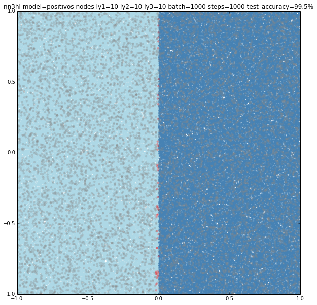
  • positivos: A trivial classification – if x>0 class=1 else class=0
  • linear: if y>x class=1 else class=0
  • circle: if (x,y) is inside a circle of radius=r then class=1 else class=0
  • ring: if (x,y) is inside a circle of radius=r but outside a concentric circle or radius=r/2 then class=1 else class=0
  • cos: if (x,y) is above a cosine with frequency=r then class=1 else class=0
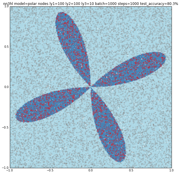
  • polar: if (x,y) is below a cosine of frequency r in polar coordinates (inside a “rose of n-petals”) then class = 1 else class = 0

The plots shown above are generated from the training sets by setting positive samples as dark blue and negative samples as light blue.

Two neural networks are defined on the code, with a single hidden layer and with two hidden layers. Several parameters may be adjusted for each run:

  • model function to use
  • number or nodes of each layer,
  • batch size and number of steps for the stochastic gradient descent of the training phase,
  • beta for regularisation,
  • standard deviation for the initialisation of the variables,
  • and learning rate decay for the second NN

Other parameters are treated as globals such as the size of the training, validation and test sets.  When the NN function is called the network is trained and tested, and the predictions are added to the plot marking them on gray if the prediction was correct and on red if the prediction as incorrect in order to see where the classifier is missing it.

You can call the NN function varying the parameters to test what happens. It’s also included some iterative code to test many variants and generate a *lot* of plots. Check the code and comment what you find.

Here are some interesting results I’ve got:

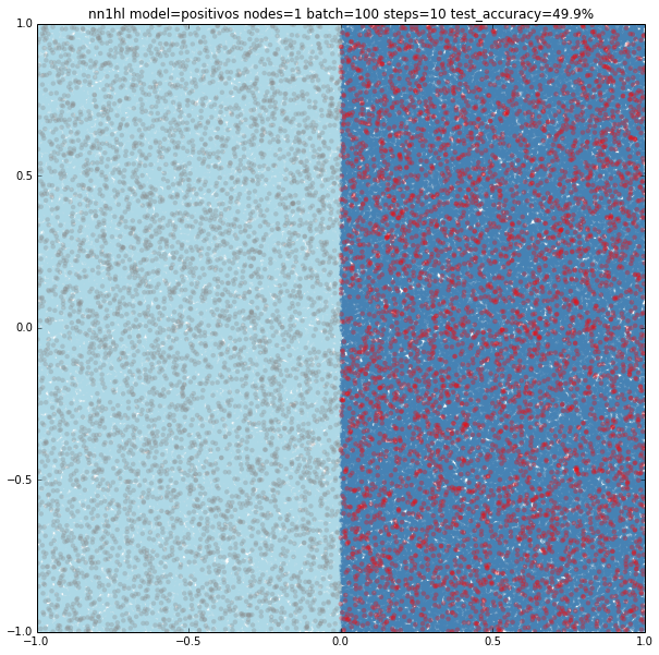
Trivial model with a single hidden node and few training data

As expected, the model is too simple to really learn anything: it’s basically classifying everything as negative and thus gets a accuracy of 49.9%


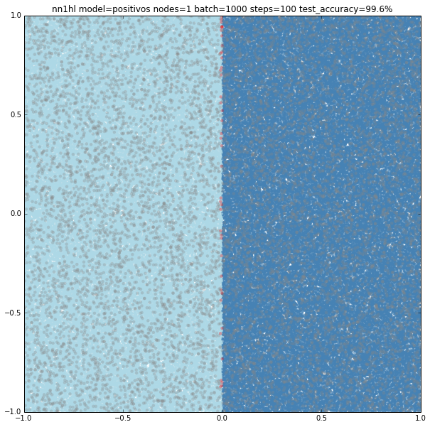
Trivial model with a single hidden node with more training data

By increasing the size of the batches and steps for the stochastic gradient descent even a single node on the hidden layer yields good results: 99.6% accuracy


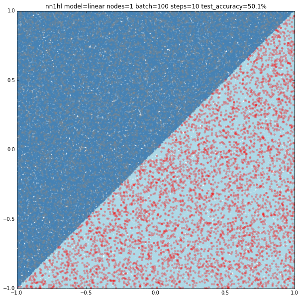
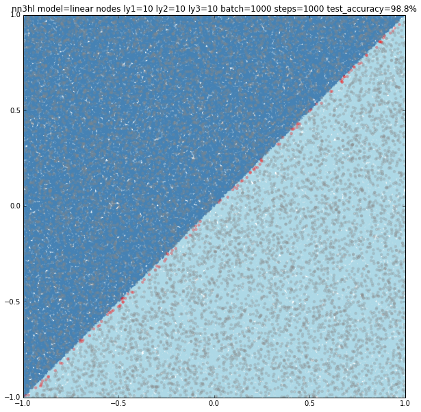
Linear model with a single hidden node and few training data

Of course few training data does anything good for a slightly more complex model: 50.1% accuracy.


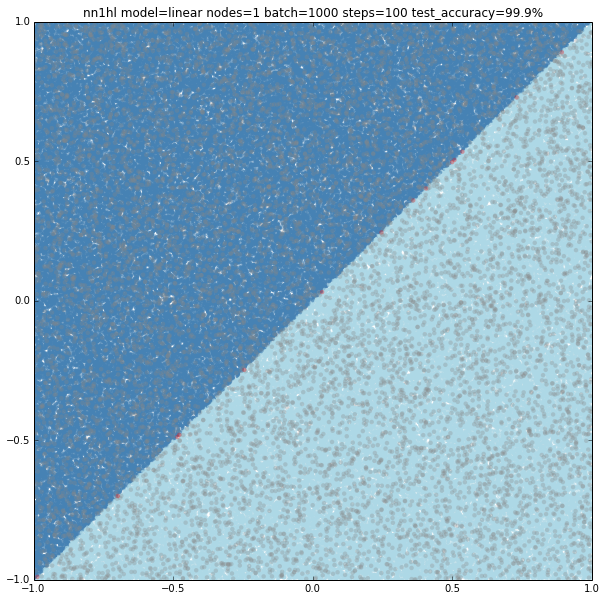
Linear model with a single hidden node with more training data

Again the classifier performs way better: 99.9%


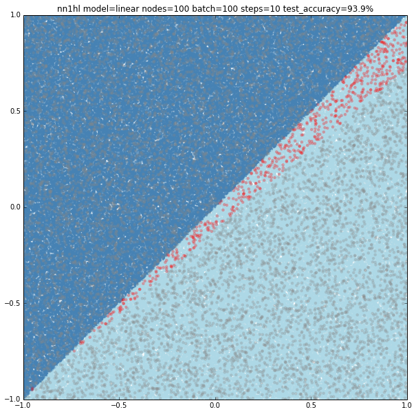
Linear model with a 100 hidden nodes with few training data

Can hidden nodes compensate for few training samples? 100 nodes, batch of 100 and 10 steps does certainly better at 93.9% accuracy and an interesting plot with linear classification on a wrong (but close) slope.


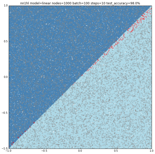
Linear model with a 1000 hidden nodes with few training data

What about 1000 hidden nodes and same parameters as before? It certainly gets you closer but not still on it: 98% accuracy. Watching the slope, one can think it may be overfitting.


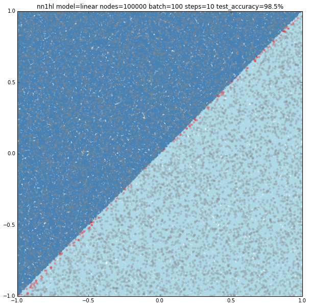
Linear model with lots of hidden nodes and few training data

First tried 10,000 hidden nodes (got 98.9%) and then 100,000 nodes (shown below) and accuracy jumped back to 98.5%, clearly overfitting. For this case, a wider network behaves better but just to a certain point.


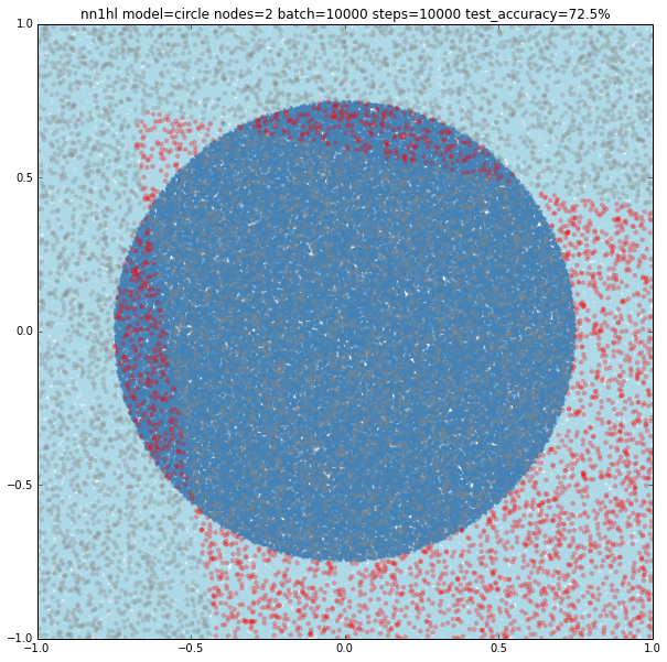
Circle with a previously good classifier

Training the classifier that previously behaved well with the circular model shows clearly it needs more data or nodes.


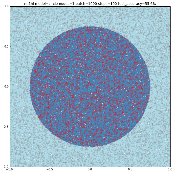
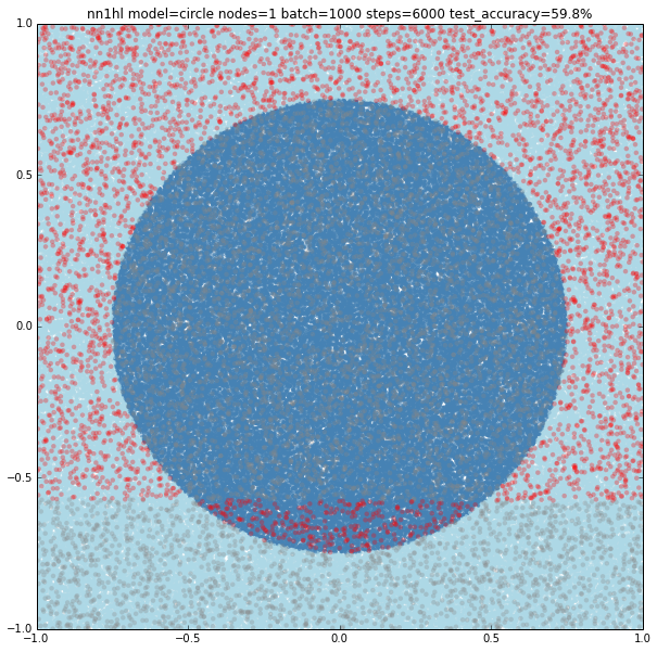
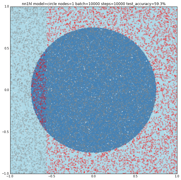
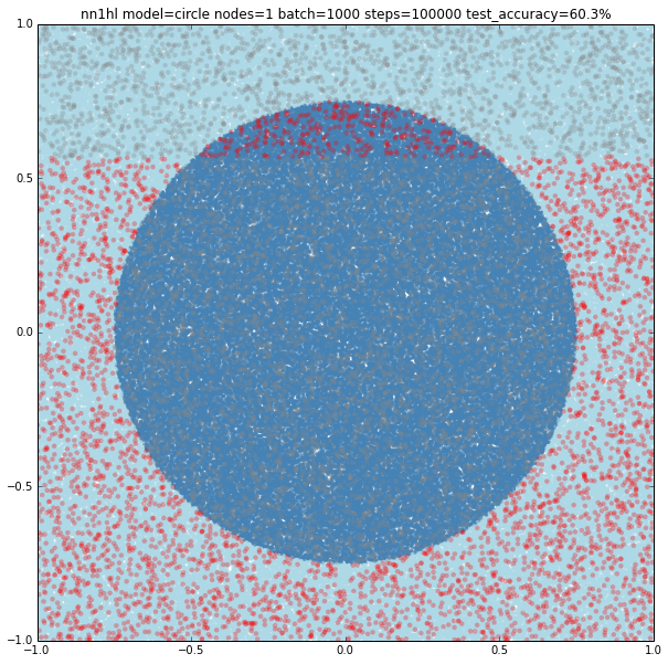
Circle with a single node

Turns out that it seems a single node can’t capture the complexity of the model. Varying the training parameters looks that the NN is always trying to adjust a linear classifier.


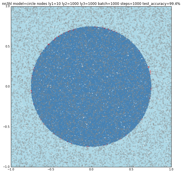
Circle with a many nodes and different training sizes
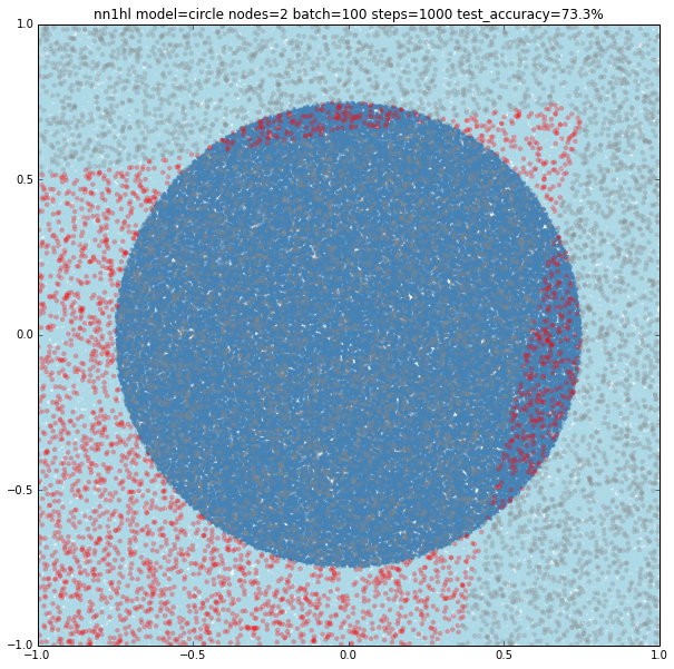
Two nodes

With two nodes the model looks like fitting two linear classifiers. Even varying the training parameters results are similar, except in some cases with more training data that looks like the last examples of single node (maybe overfitting?)

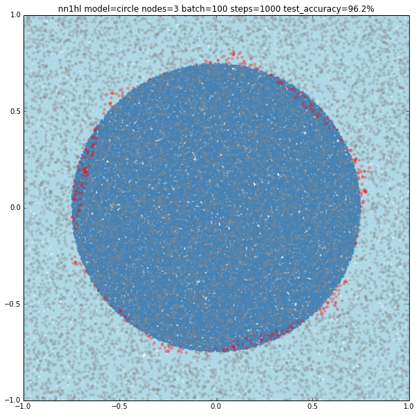
Three and more nodes

Using three nodes things become interesting. For a batch size of 100 and 1000 steps the NN gives a pretty good approximation to the circle and goes beyond adjusting 3 linear classifiers. Something similar happens varying the training parameters.


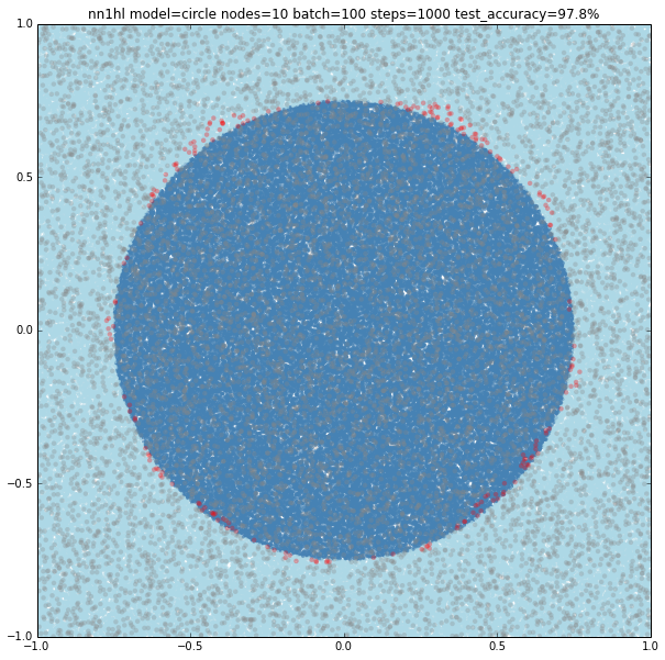
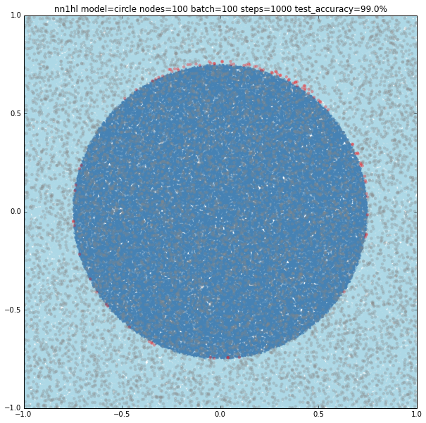
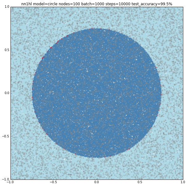
Increasing the number of nodes increases the precision and the visual adjustment to the circle. Check for 10 (97.8%), 100 (99%) and seems to stop at some point 1000 (99%)
 

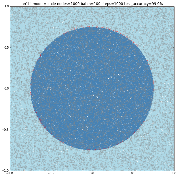
Finally increasing the training parameters on the best classifier gives us a nice 99.5% accuracy, but not sure if it’s overfitting
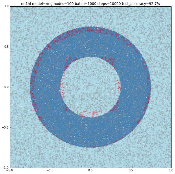
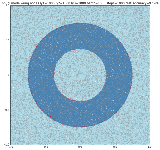


The Ring

For the ring I started testing one of the best performers on the circle: 100 nodes, batch size of 100 and 1000 steps. Somehow expected, it tried to adjust to a single circle and missed the inner one.


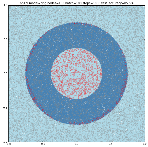
Increasing the training parameters gave an interesting and unexpected result:


I also found that running many times with the same parameters may yield to different results. Both cases could be explained by the random initialisation and the stochastic gradient descent as the last example looks like a local minimum. Check below another interesting result using the exact same parameters yielding a pretty accurate classifier (92.7%)


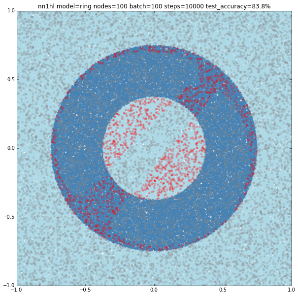
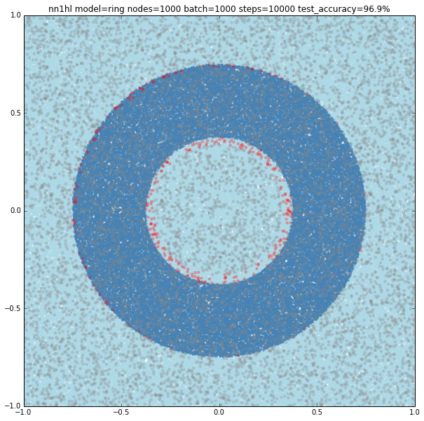
Increasing the number of nodes and the training parameters improves accuracy and makes more likely to get a classifier with a pretty good level of accuracy (96.9%). Shown below, 1000 nodes, batch size of 1000 and 10000 steps.
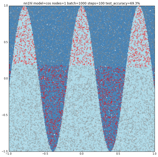
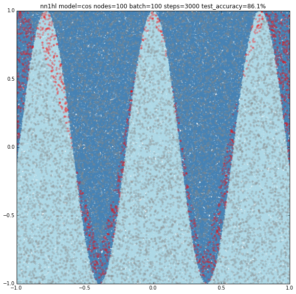
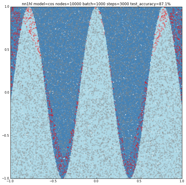
Cosine

With few nodes and different training parameters we see the classifier struggling to fit.

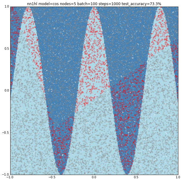
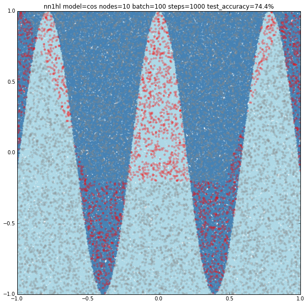
Increasing the parameters gives a model that doesn’t increase very much the accuracy (around 87%). From the ring and the cosine it looks like there are limits to the complexity a single hidden layer can handle.

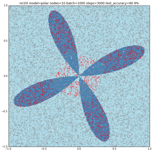
Cosine in polar coordinates

This example came as a way to try a harder problem for a classifier. As expected, the most basic versions of the parameters yield bad results. Just keep in mind that a trivial classifier that labels everything as negative would have about 80% accuracy.


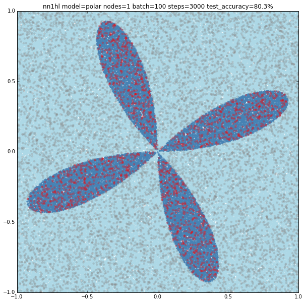
We can see that a NN with 10 nodes tries to adjust a central area as positive. Results are bad but we can see what the NN is trying to do. Increasing to 100 nodes give very similar results.


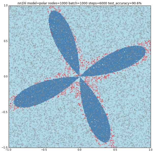
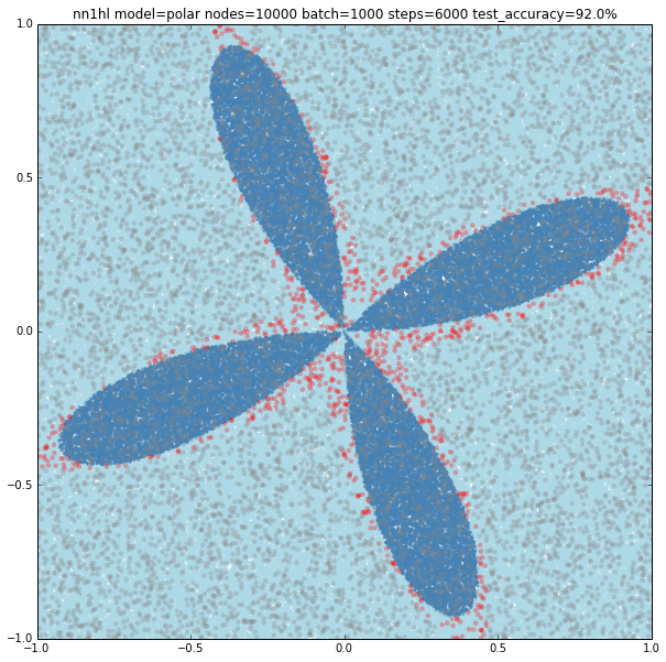
With 1000 nodes the classifier improves accuracy but misses big on the center of the model. But going up to 10,000 nodes does not improve much more. This makes me think that, as with the case of the rectangular cosine, there is a limit on what a single layer neural network may model for the classifier, and that more complex distributions may need a different kind of network.


A deeper neural network

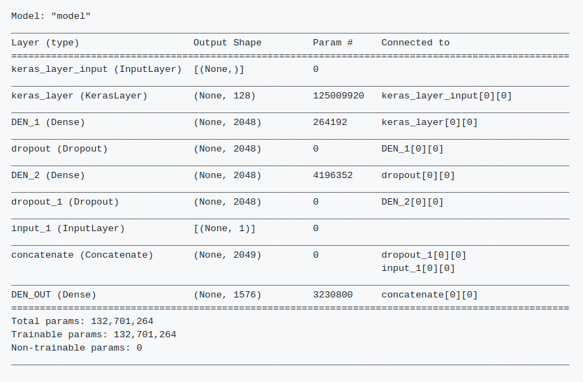
Next I was interested in what happens with deeper networks, expanding the exercises from the Udacity course to a 3 layer NN and testing with the same models.
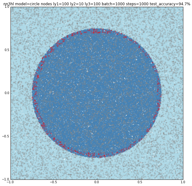
First finding was that for the Positivos example the NN needed to be of at least 10 nodes on each layer to get good results. Same classifier also worked well for the linear model, but not with the circle.


The circle needed quite an amount of nodes in some of the layers to get over 99% accuracy. The simplest model I could find with a 99.4% was (10,1000,1000) nodes. Other models with a similar count of nodes gave similar results. Models with less nodes failed completely or gave increasing accuracies.


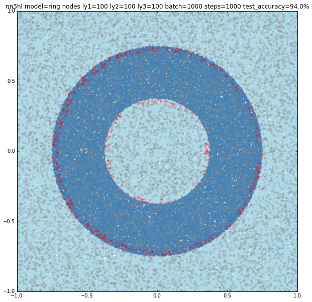
Interestingly, the ring also converged faster with (100,100,100) nodes with a 94% accuracy up to a nice 97.9% accuracy for a (1000,1000,1000) configuration.


The cosine also improved with the deeper network achieving a 94.3% accuracy with a (1000,1000,100) network. What is also interesting is that models learned by the deep network approached better than the wide network almost from the beginning. If you want to check, run the iterative version you can find commented on the code.

The Polar Cosine and Deep Network

The most interesting case is the polar cosine on the deep network as it looks like a really hard classification problem. Base accuracy is about 80.3% for the all negative classification. As we grow the number of nodes in the different layers interesting patterns appear as you can see in the examples below.

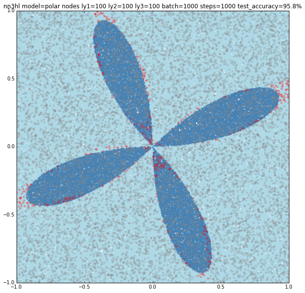
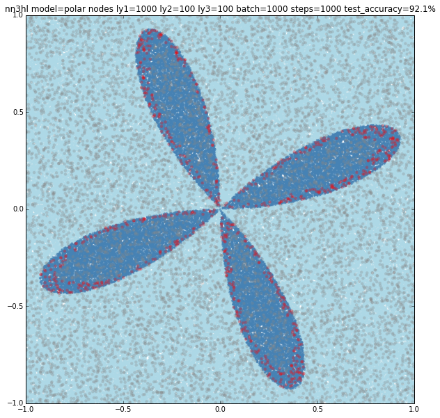
The last example does a pretty good job classifying this complex model with a 98.1% accuracy with the three layers and 1000-1000-1000 nodes.


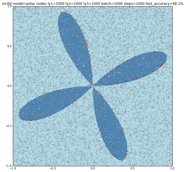
I find very interesting seeing how the wide neural network seems to have a limit on the complexity of the classifier it can learn. And the deep network looks like being able to capture that complexity. Check the Jupyter notebook at Github. You will need Tensorflow installed to run it.

Detecting Whales: Kaggle Right Whale Recognition Challenge

Fork on Github
Kaggle’s NOAA Right Whale Recognition Challenge aims to develop an algorithm to identify individuals of Right Whales, which are critically endangered. It is a great chance to study machine learning and digital image processing although looks to me as a really hard challenge. Anyway I’ve developed this method to detect the whale in the photograph and I’m releasing it in a hope that it may help others.

It takes advantage of the fact that most pictures are pretty plain, with almost all of the area covered by water, and have a smaller region of interest which corresponds to the whale, so the histogram for most of the image will be similar except on the region of interest. The algorithm looks recursively to subimages that have an HSV histogram not similar to the original image’s histogram, marking those regions in white and else on black. Then searches for the biggest continuous region using contours and places a bounding box around it, assuming it’s the whale. The image is called “extract” and is saved along the black & white mask.

Check the code in Github. Uses Python 2.7 and OpenCV 3.0.

Original Image:
whale

Whale found:
whale

Areas found mask:
whale

ROI Mask:
whale

ROI Extract:
whale